Blog

In our February 2021 blog post The value of visualisation in improving data quality: Mapping MEI, we already discussed valuable insights that can be gained by visualising data from CERL resources on a map. In the following blog post, we add to these insights by describing another approach to visualising metadata. This time, by creating networks of places from the CERL Thesaurus, we are able to illustrate both geographical places themselves as well as connections between them.

The CERL Thesaurus (CT) contains nearly 1.5 million records, around 36,500 of which are geographical places such as London, Paris, or Stockholm. Other CT records (as well as data sets outside of the CT) can be linked to these geographical places, e.g., as place of birth, place of death, or place of activity. Links between CT records are displayed in the CT web interface as direct hyperlinks, allowing for an easy navigation between related records.

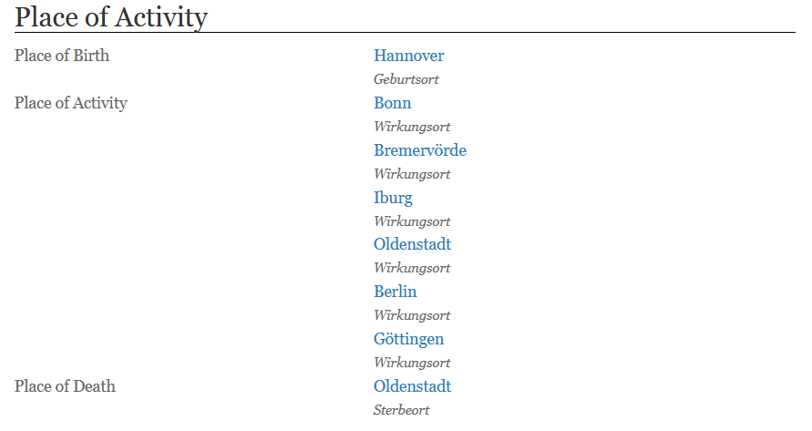
Figure 1: Geographical places linked to a person‘s record in the CERL Thesaurus

Additionally, based on these hyperlinks, an overview of ‘Related Records’ is generated automatically for every geographical entity in the CT’s web interface.

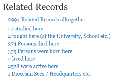
Figure 2: Related Records from a geographical entity in the CERL Thesaurus

However, this section of the website does not reflect all knowledge implicitly contained in these links. Although we might already get an idea of the putative importance of a city (in terms of the number of people and institutions that resided, worked, lived here), a key piece of information is missing: the relationship between a place and other places.

Let’s illustrate this with an example. Imagine you are interested in the role a certain city played during the early 17th century. How many people were active in this city? Did they also work in other cities afterwards? Did they come back? How did this change over time?

The absolute number of people that were active in a city (as currently shown in the web interface) is already a good indicator but does not allow for many conclusions. Looking at Fig. 2, we can see that the number of people linked to a city can easily exceed some thousands. It would be a strenuous activity to look at all these records individually just to find out if a person lived there during the period of interest. If you are familiar with using the CT search syntax, you might be able to express your information need in a complex query by formalising find all records of type „person“ where the biographical dates are within XXXX and YYYY and where the person was either active, lived, or studied in the city represented by record identifier XYZ. Possible, but quite complex.

To make matters worse, even if you could manage to get a list of all people in question you would still have to go through each of them to find out which other places they worked or lived in. Only after having compiled all these data you would be able to visualise the networks around your city of interest.

This is where we can benefit from network analysis. Basically, a network is simply a collection of nodes and edges between some of these nodes. With this in mind (and a full CT export at hand), we can convert data from the CT into an edge list – a data format that allows for representing network data in an easily readable way by listing two cities and the number of CT records in which both cities occur. If they occur in at least one record, an edge can be drawn between these two cities. These cities can be seen as somewhat ‘similar’ or ‘connected’.

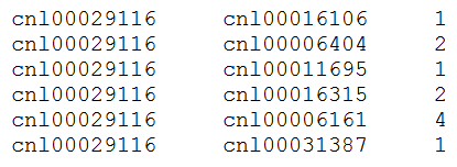
Figure 3: Mutual occurrence of CT record ID „cnl00029116“ (Antwerpen) and six other cities

The creation of this edge list is based on an analysis of each record that represents a person in the CT and its links to cities from the CT, as shown in Fig. 1. If we are only interested in a subset of the full CT – e.g., only a certain period of time – we can filter the records in advance. For example, we could incorporate only those records of people that lived during the early 17th century (let’s say, between 1600 and 1625). Naturally, this filtering relies on the quality and availability of the underlying data. With our (filtered) edge list, we can then draw a network visualisation.

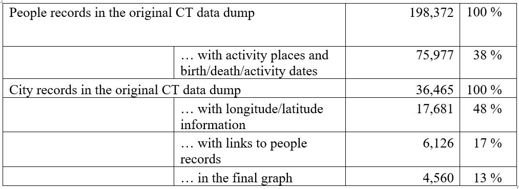
As is so often the case, things are not as easy as they seem. Since we are concerned with geographical data, drawing a network of cities is almost only meaningful if we are able to place the cities in the correct position on a map. That’s why we also choose to export all longitude/latitude coordinates for each city in the CT. Note that in our final network, we are thus only able to show those cities where these coordinates are available in the CT (that is 48% of the records, see table below). Additionally, since a city might have multiple IDs in the CT and links from person records may therefore refer to a number of different IDs to refer to the same city, we need to map all these IDs to a single unique identifier for each city.

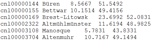
Figure 4: Longitude and latitude of cities from the CERL Thesaurus

A few other decisions have to be made: e.g. what part of the world do we want to visualise – a single country, a continent, the whole world? Do we consider only cities with edges – or also those that do never occur together with other cities? How big do we draw edges and nodes, and in what color? Answers to these questions do not only depend on the research question we have in mind, but also on the readability and size our resulting network visualisation should have. Moreover, questions like these show that constructing a meaningful visualisation is not a trivial task since there are a lot of situations where the decision for or against something might lead to the incorporation or omission of (potentially relevant) data. As impressive and convincing visualisations may be – it is always of paramount importance to also accurately describe the decisions that led to their construction.

Having said this, we can now draw one of many possible networks: cities located on a map of modern Germany and their mutual occurrence in the CT in the year 1650. The size of a city’s node (the blue dots in the image below) gives an indication of the number of its connections with other cities.

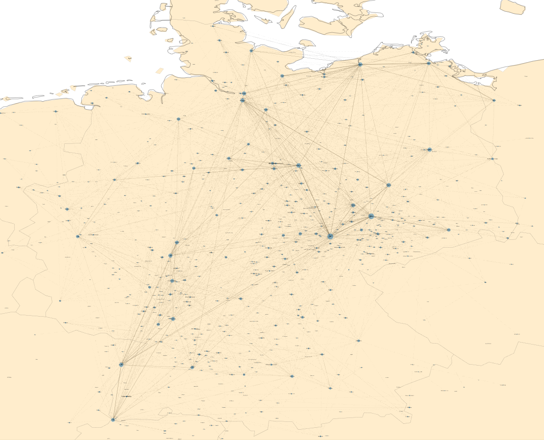
Figure 5: German cities and their mutual occurrence in the CERL Thesaurus in the year 1650

A look at the full network already allows for the identification of some places with high importance (Jena, Leipzig, Helmstedt etc.). Zooming in can further support the identification of patterns, outliers, central nodes, or hubs. For example, there is a quite important city named ‘Wittenberg’ near Hamburg, whose importance seems to be the result of many wrong links that should actually refer to Wittenberg in Saxony.

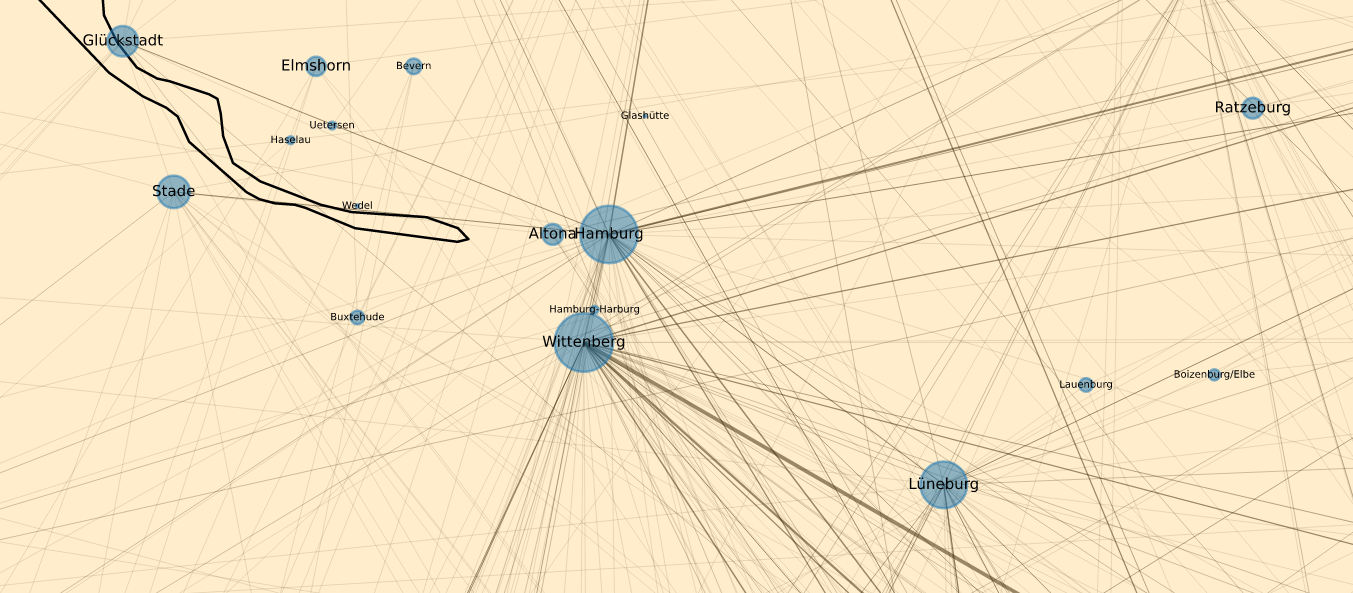
Figure 6: Wittenberg near Hamburg – the result of wrong links?

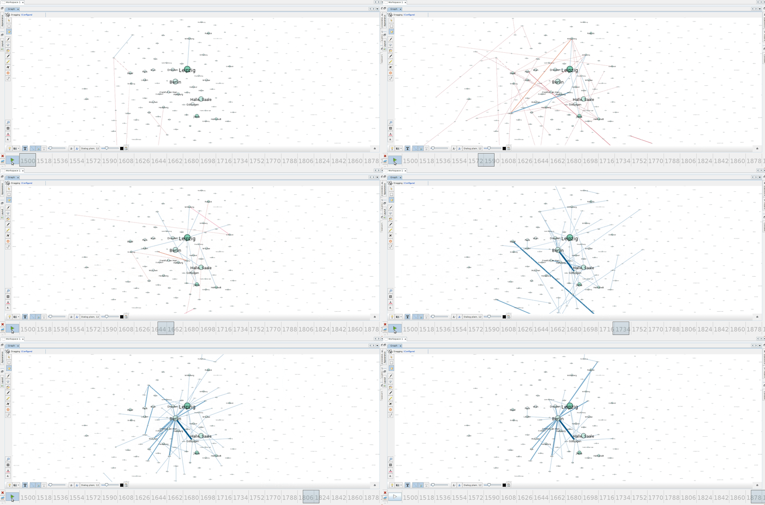
There are a lot of network analysis tools out there, most of which can handle standard network representation formats. With only some minor additions to our source code, we can convert our data used for the above network into a format that, e.g., can be used with the software Gephi. In Gephi, it is quite easy to generate dynamic network animations, which allows us to carve out the evolution of city networks over time (e.g., observe the increasing importance of Berlin starting around the year 1700 and see how Helmstedt becomes quite insignificant near the end):

Based on the plethora of possible networks that can be generated from the CT – on different maps, for different years/decades, including only people with certain professions etc. – many analyses are possible, and thus, the improvement of data quality, the discovery of meaningful relations, and the visualisation of what’s actually in the Thesaurus can be supported.

However, it is important to note that all networks and visualisations can only be as good as the data they represent. If we take our network of cities as an example: not all people records in the Thesaurus contain information about activity places, some do only list the place of birth and/or death or even no places at all. Many records do not contain information about the time a person lived and thus had to be excluded from our analysis. Last but not least, city records without longitude/latitude information could also not be used in creating the network visualisation on a map. To give an idea of the data that are theoretically available and those that are extensive enough to use them, have a look at the following table:

To simplify our analyses, make them more structured and allow for a better reusability, we started developing a Python library named Bibliometa. A tutorial that uses Bibliometa with sample data from the CERL Thesaurus can be found on GitHub. If you are working with data from the CERL Thesaurus yourself and want to share your results and/or scripts, feel free to contact us. We would be happy to include your work into the Python library and tutorial.

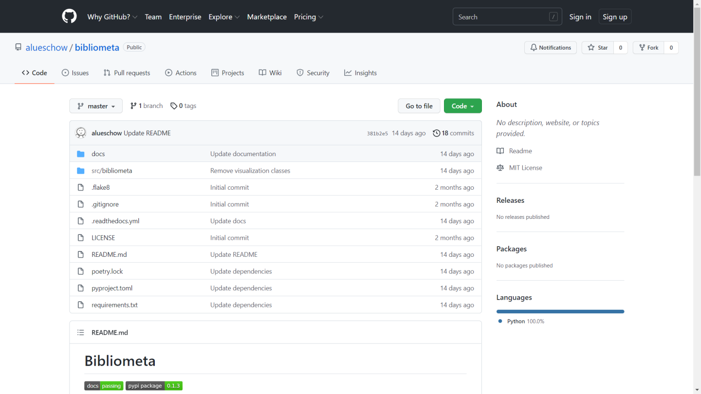
Figure 7: Bibliometa